Time-binned correlation¶

The Time-binned correlation method is designed to calculate correlations from the time-binned fluorescence signal. The input data should be provided as single-column files containing integer values, where each row corresponds to the number of registered photons. The interface layout of this method is similar to the previously described Import PTU. One limitation of the method concerns the size of the time-binned time-trace files. In contrast to the TTTR data format (e.g., .ptu files), the time-binned data includes all time points, including those without signal. This means the files can reach enormous volumes, making them difficult to analyse, especially on slower CPU machines.

Import uncorrelated data¶

In the file menu, click Open single-column data directory. It will start the dialogue window where you can select the folder containing your time-trace data. The software reads the time-trace data stored in the .txt files. For single-fluorescence-channel data, the file name does not matter except for the .txt extension. If the folder contains two-colour data, the file names should correspond to the channel. For example, some_name_c0.txt and some_name_c1.txt files correspond to data from channel 1 and channel 2, respectively. After importing the two-colour data, the file names will be displayed in the file list only as some_name.

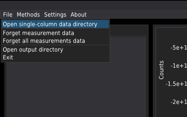
After opening the data folder, the program will prompt you to select the output data folder. Press Yes to create the output subfolder in the same folder as the time-trace data are located. Press No to select the output folder manually.

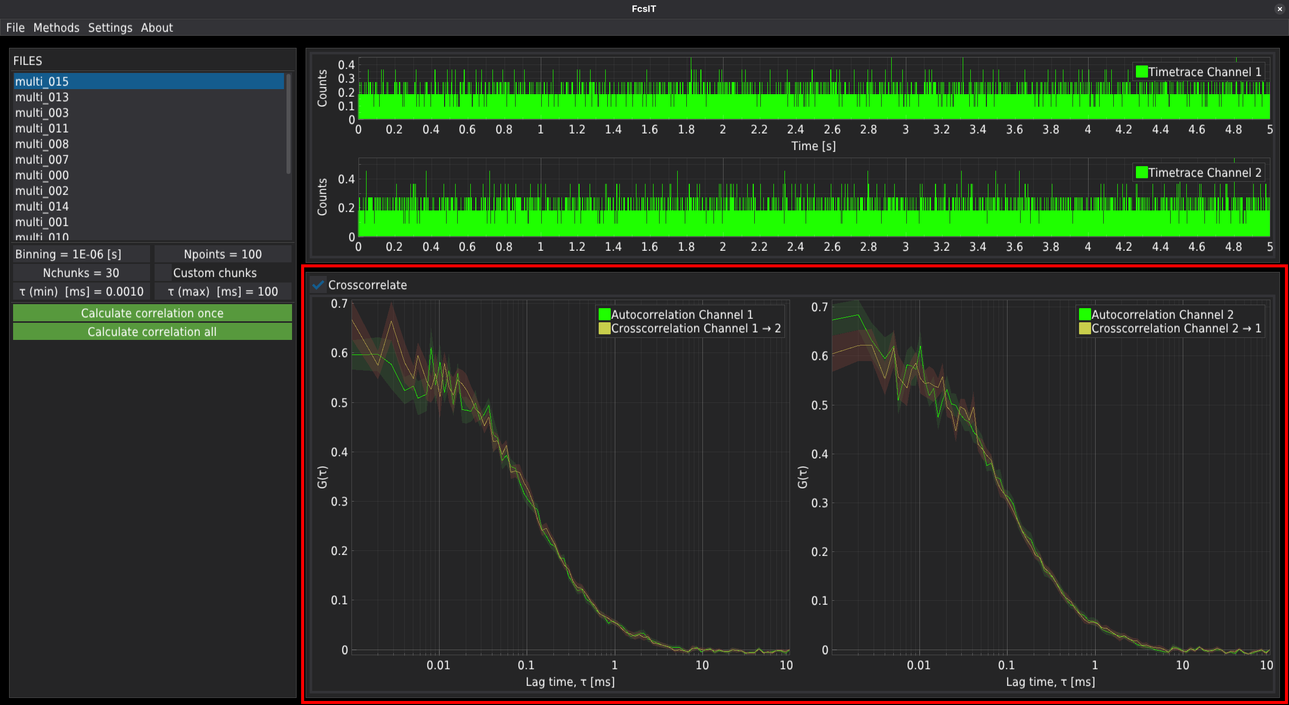
The time-trace plots¶

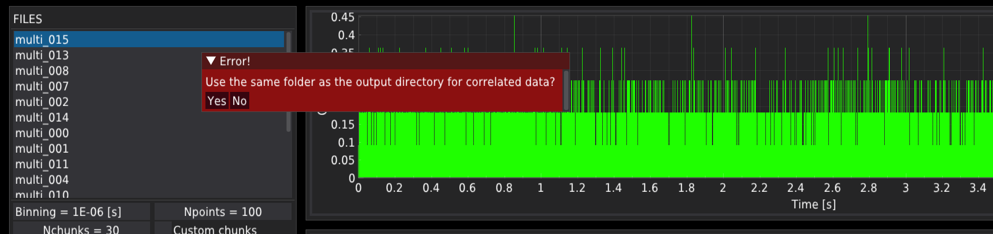
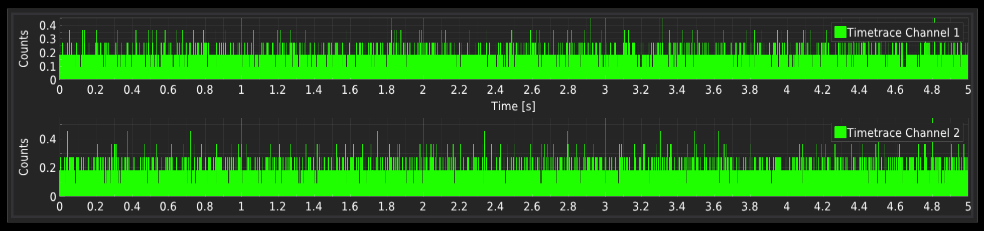
The fluorescence time-trace signal is displayed in the top centre part of the window as:

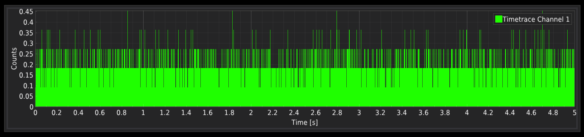
or

The correlation control panel¶

The correlation control panel has a similar form to that in the Import PTU module. The main difference is in the field responsible for binning the time-trace data; see below.

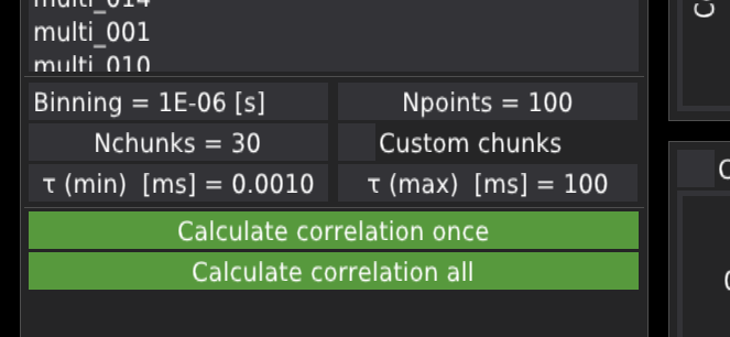
• The Binning field defines the time step or in other words the bin lenght in the imported timetrace data. !!!CAUTION!!! This field is always user defined and directly influences the resulting coorelation curves. After clicking, the user need to provide the time resolution. Note the resolution should be given in the exponential notation in seconds, where 1e-6s = 1$\mu$s.

• The Npoints field defines the output number of points in the correlation curve.

• The Nchunks field defines the number of chunks to which the whole time-trace signal is divided. The chunks are used to determine the mean and standard error of the mean for each lag-time point along the correlation curve; for details, see the preprint Kalwarczyk (2026). By default, the time-trace is divided into thirty evenly distributed chunks.

• The Custom chunks checkbox activates/deactivates user-defined chunks. When activated, the draglines and green fields appear on the time-trace plots. The user can unselect part of the signal that won’t be included in the analysis. The length of chunks influences the calculated maximum lag-time of the correlation curve.

• The Tau (min) field defines the minimal lag-time of the correlation curve.

• The Tau (max) field defines the maximal lag-time of the correlation curve.

The correlation plots¶

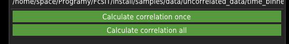
By pressing the Calculate correlation once button, the correlation curve(s) will be calculated and automatically exported to the output subfolders just for a single selected file. Pressing the Calculate correlation all button performs the same operations on all files in a folder.

The correlation curves are displayed in the central pannel.