Import PTU¶

The Import PTU method extracts the data from the binary .ptu files containing the TTTR data, acquired with the SymPhoTime software (PicoQuant Germany). This module allows the user to filter TCSPC data using time gating and/or statistical filtering based on fluorescence-lifetime decay. It is also possible to exclude the unwanted parts of the time trace and correlate the fluorescence fluctuation signal. Below there is a detailed workflow for using the Import PTU module.

Import PTU files¶

The software recognises all .ptu files in the given folder. The user is advised to consolidate all _.ptu_files related to the given experiment into a single folder. Press Open PTU files directory in the File menu to open the folder.

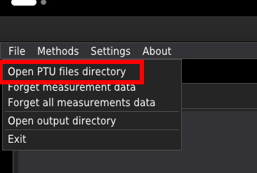
In the pop-up window, select the folder where you store your data. The list of files in the chosen directory will appear in the list box at the top-left of the window.

The time-trace plots and the correlation control panel¶

The time-trace plots¶

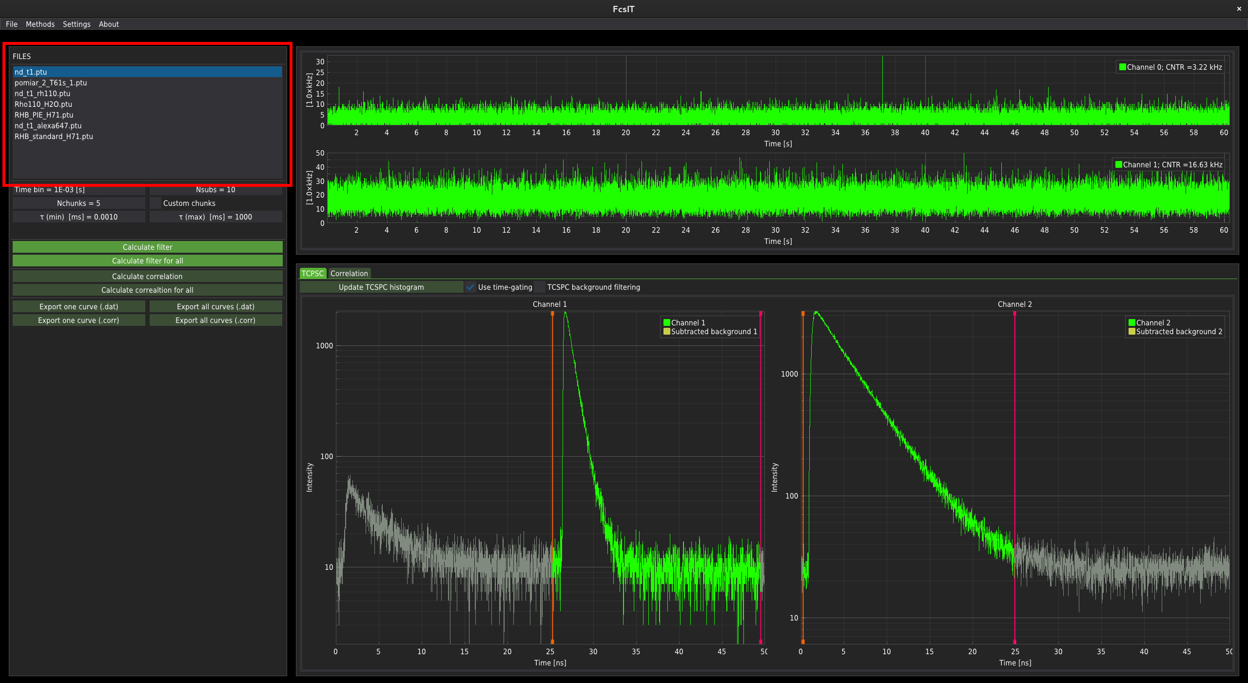
The fluorescence time-trace signal is displayed in the top centre part of the window.

For data with a single fluorescence channel, only one plot is displayed. For two channels, the two separate time-traces are plotted. In the control panel on the left-hand side of the window, below the list of files, the correlation parameters controllers are located.

The correlation control panel¶

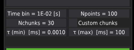
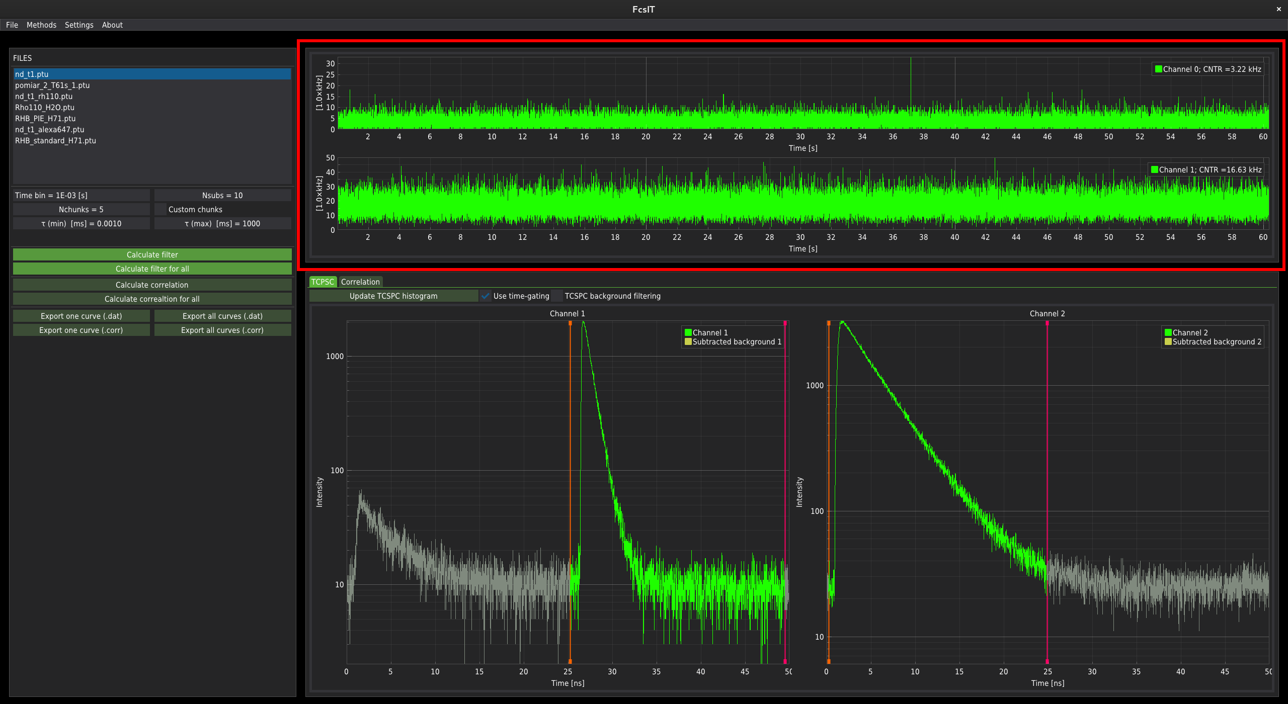
• The time bin field changes the time resolution in which the time-trace signal is being displayed. Its value does not influence the correlation data. After clicking, the user can provide the time resolution. Note the resolution should be given in the exponential notation in seconds, where 1e-3s = 1ms.

• The Npoints field defines the output number of points in the correlation curve.

• The Nchunks field defines the number of chunks to which the whole time-trace signal is divided. The chunks are used to determine the mean and standard error of the mean for each lag-time point along the correlation curve; for details, see the preprint Kalwarczyk (2026). By default, the time-trace is divided into thirty evenly distributed chunks.

• The Custom chunks checkbox activates/deactivates user-defined chunks. When activated, the draglines and green fields appear on the time-trace plots. The user can unselect part of the signal that won’t be included in the analysis. The length of chunks influences the calculated maximum lag-time of the correlation curve.

• The Tau (min) field defines the minimal lag-time of the correlation curve.

• The Tau (max) field defines the maximal lag-time of the correlation curve.

The TCSPC plots, data filtering and correlation plots¶

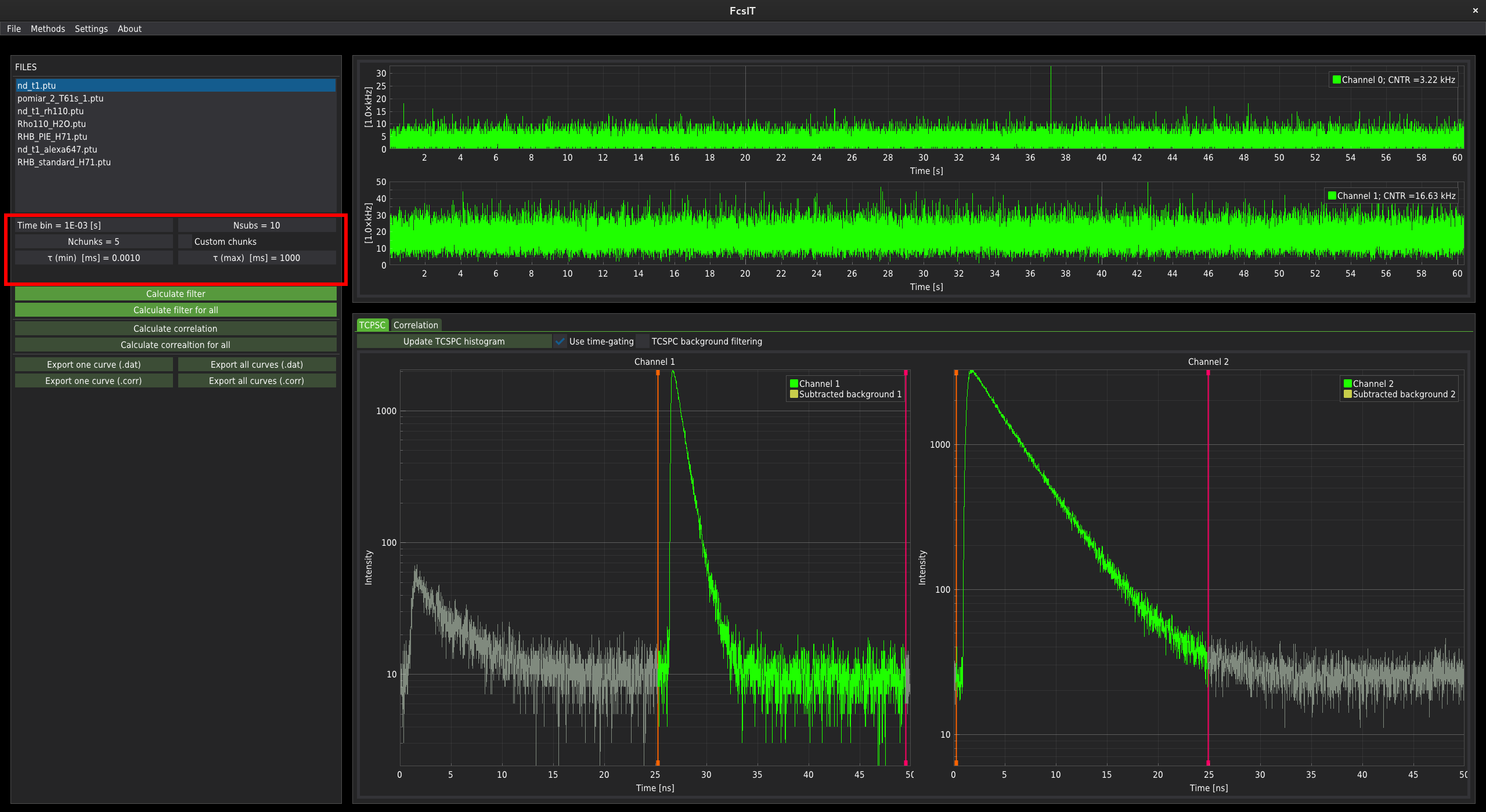
Below the time-trace plots, there is a window with the TCSPC histograms and Correlation tabs, each containing one or two plots, depending on the number of channels in a given .ptu file.

The TCSPC plots and data filtering¶

By default, the TCSPC tab is active at startup.

First, the imported .ptu file needs to be filtered. The filtration method can be selected by checking/unchecking the checkboxes Use time-gating or TCSPC background filtering.

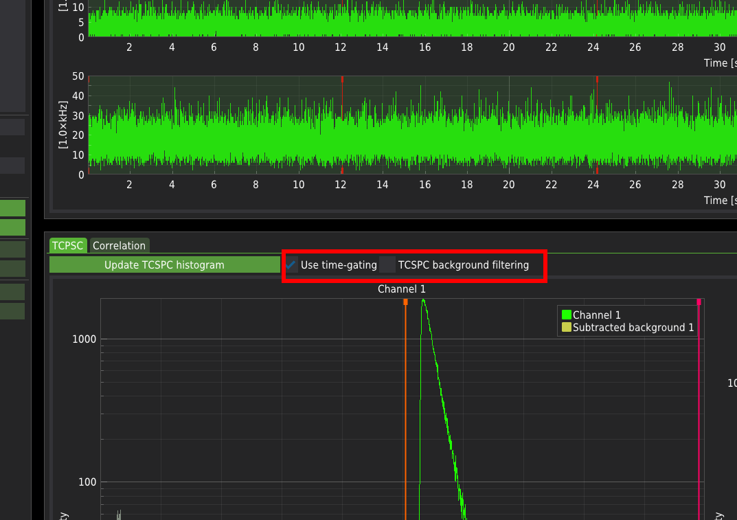
• Use time-gating enables the selection of the part of the TCSPC histogram that will be included in the analysis. The active part of the signal is marked in green. The photons that fall into the inactive range of the histograms (grey parts of the plots marked in grey) will not be included in the analysis. The software recognises whether the measurement was performed in the PIE mode and automatically adjusts the predefined ranges to those dedicated to specific PIE lines. The vertical drag lines on the TCSPC histograms determine the user-defined time gating.

• TCSPC background filtering uses the algorithms and methods described in the literature: Enderlein & Gregor (2005), Kapusta et al. (2007). The level of background taken into account during filtering can be selected by moving the horizontal drag line on the TCSPC histogram.

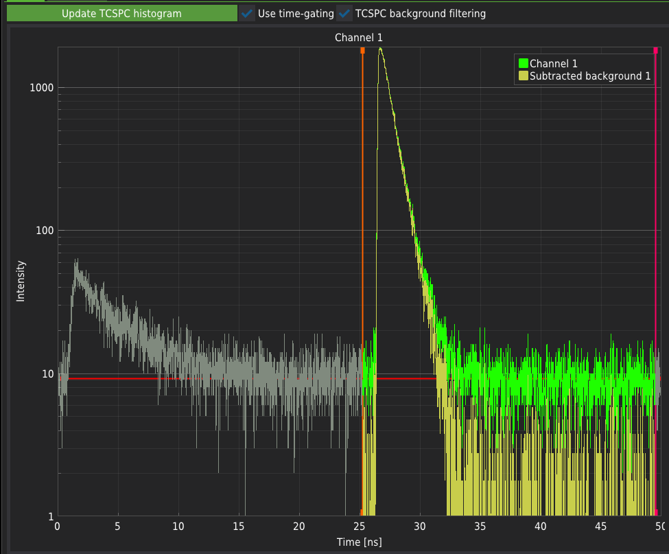
• Selecting none of the checkboxes will result in an unfiltered signal. For typical FCS measurements, both checkboxes must be selected.

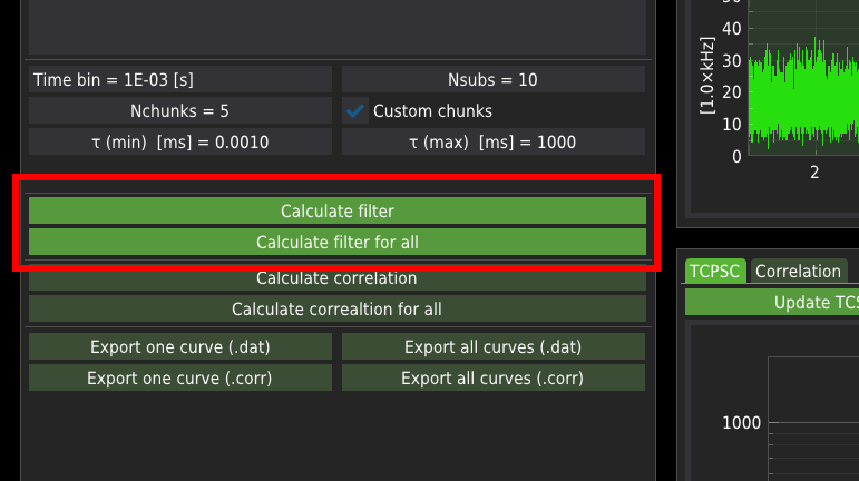
Press the Calculate filter button to calculate the filtering masks for a single file only.
Press Calclulate filter for all button to calculate the filtering masks for all files from the list.

The Correlation plots¶

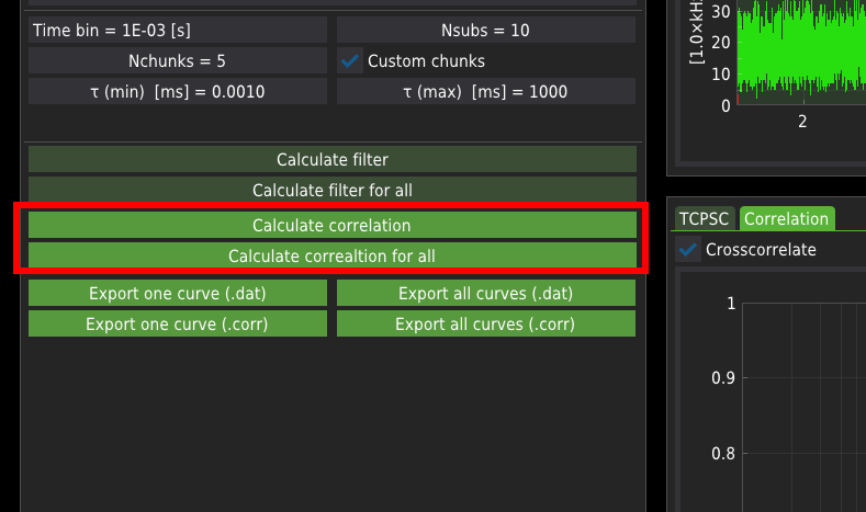
Once the filters are calculated, switch to the Correlation tab.

Press the Calculate correlation to calculate correlation curves for a single file.
Press the Calculate correlation for all button to calculate correlation curves for all listed files.

Export correlation curves¶

The calculated correlation curves can be exported either for a single file or all files at once. The FCS curves are exported in one of the following formats:

• .dat is a raw ASCII file containing three columns: the correlation time axis, correlation values, and the corresponding standard error

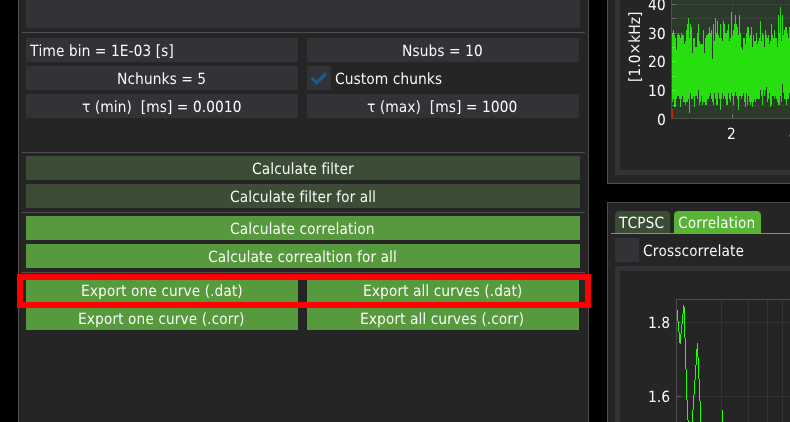
• .corr format is a binary format consisting of the same data as in the case of the ASCII files. Additionally, the .corr files include the average count rate (averaged across all chunks) and the correlation curves calculated for each chunk. The mean count rate is particularly useful for calculating the molecular brightness of the probe when fitting with the FCS fitting module.

The exported corralation curves will be stored in four separate folders automatically created in the user-defined folder. The folders are named as:

• AutoCorr_ch1 - Autocorrelation data corresponding to channel 1,

• AutoCorr_ch2 - Autocorrelation data corresponding to channel 2 (if available),

• CrossCorr_ch1 - Crosscorrelation data between channels 1 to 2 (if available),

• CrossCorr_ch2 - Crosscorrelation data between channels 2 to 1 (if available).