FCS fitting
The FCS fitting method is designed to fit the correlated fluorescence correlation spectroscopy (FCS) data.
Importing the data files
The software reads files containing correlation data from a given folder. It is therefore recommended to keep the correlation data for a series of measurements in a single folder. The software reads several file types, and each has its own position in the File menu.
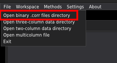
The .corr file type is the most preferred. It is a binary pickle file containing the correlation data, the count rate registered for a given file, and the correlation data for each chunk. The files of this type are generated in the Import PTU method. Click on the Open binary .corr files directory in the File menu to read all the .corr from the selected directory.
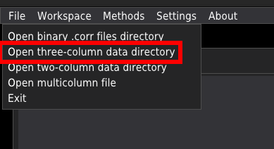
The .dat files containing the tab-separated three-column data (time, correlation, and the correlation error). Those files can be obtained by exporting the correlated data from the acquisition software (tested with SymPhoTime64 from PicoQuant). To import the folder containing the files, click the Open three-column data directory in the File menu.
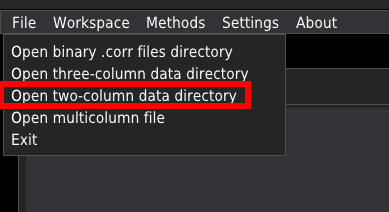
The .dat files containing the tab-separated two-column data; time, and the correlation data. To import the data folder, click Open two-column data directory in the File menu.
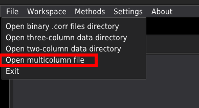
The .dat files containing multicolumn data. for example, the SymPhoTime64 software allows the export of many correlation curves as a single file. Clicking the Open multicolumn file loads the multicolumn file, creates the folder of the same name as the opened file with the addition of ‘_curves’ string at the end of the name, and saves each of the curves into a separate three-column file. Finaly all isolated files are imported into the fitting module.
Selecting and adding models
Selecting the model
At the top of the central window, there is a droplist to select the mathematical model to fit the FCS data. A detailed description of each available model is given in the Fitting models section.
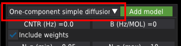
Once the model is selected, the set of new fields related to the fitting parameters will appear below the model selection panel.
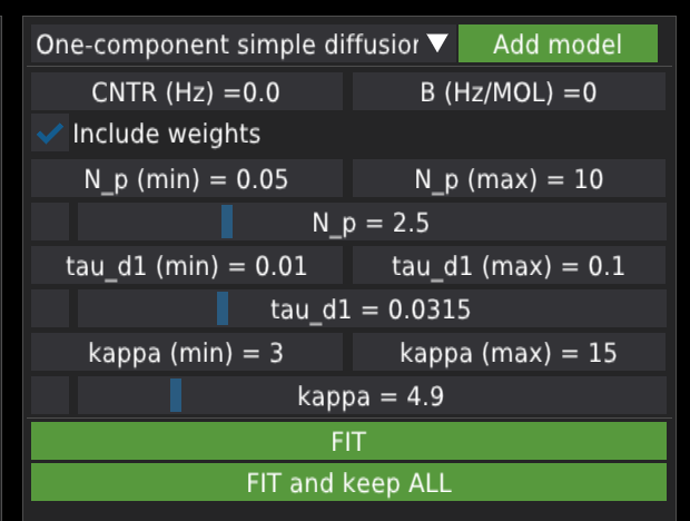
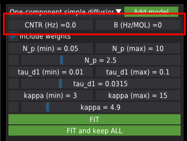
The first row of the list corresponds to the count rate and the molecular brightness, , given in Hz per molecule. is calculated from the value of countrate and the mean number of molecules in the focal volume .
Below, there are fields related to model variables. Each variable has four fields: the minimum value, the maximum value, the fixed checkbox, and the value slider. The minimal and maximal values provide the fitting algorithm with a range to search for the solution. The user can change the values by double-clicking, Ctrl+clicking, or dragging with the mouse. The fix checkbox is located in the lower row of each variable’s section on the left-hand side of the variable’s value field. When checked, the fitting algorithm will keep the variable constant. The value slider defines the initial value of the variable used for fitting. The user can move the slider to pre-adjust the initial fitting value. Pre-adjusting is strongly advised, especially when the models have many variables, as this can make the fitting algorithm unstable and lead to errors. After fitting, the value slider will display the fitted value.
Adding a new model
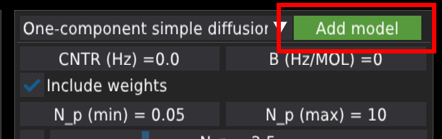
The user can add a model manually by clicking the Add model button, which opens a pop-up window to define the model.
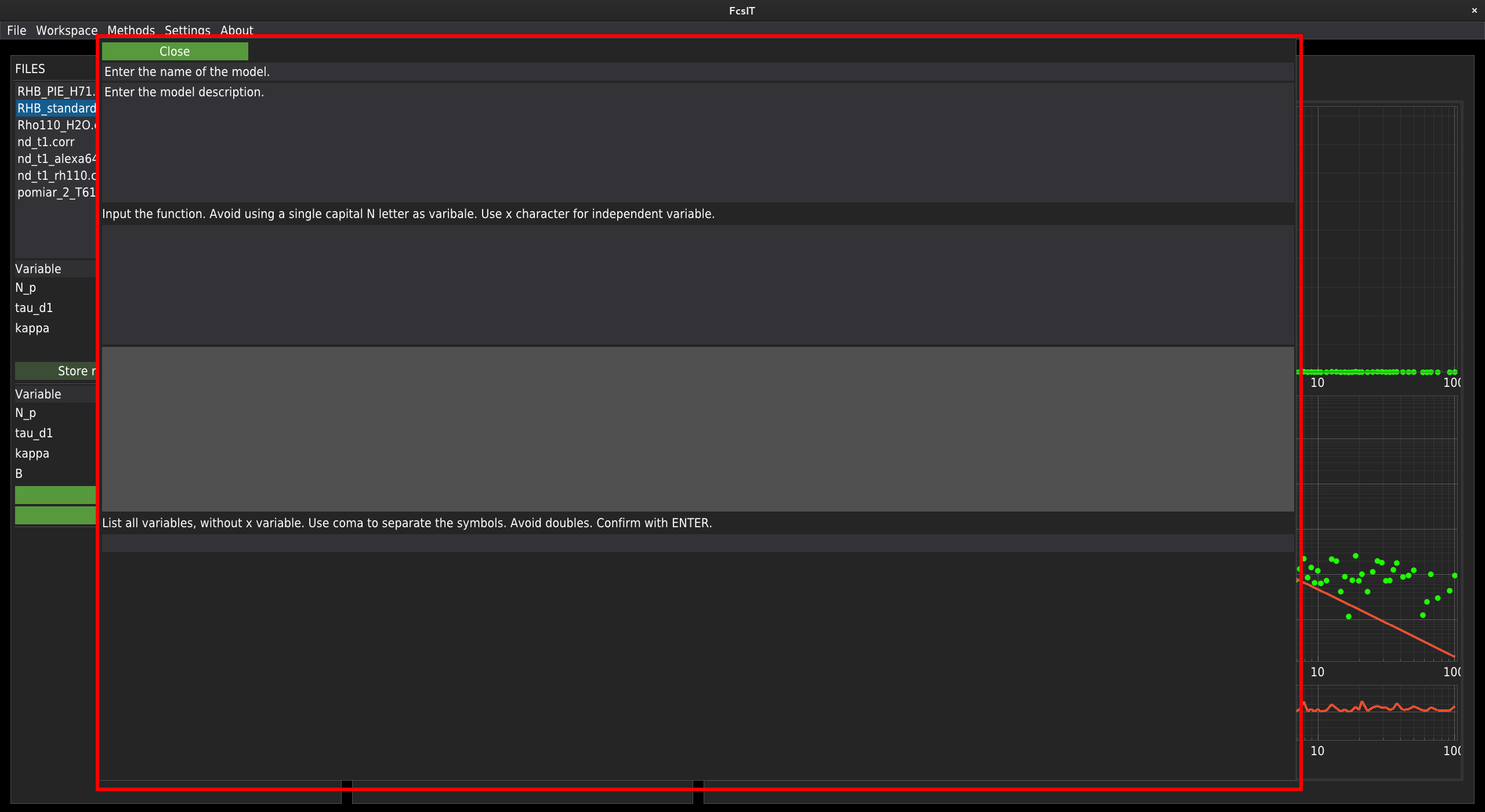
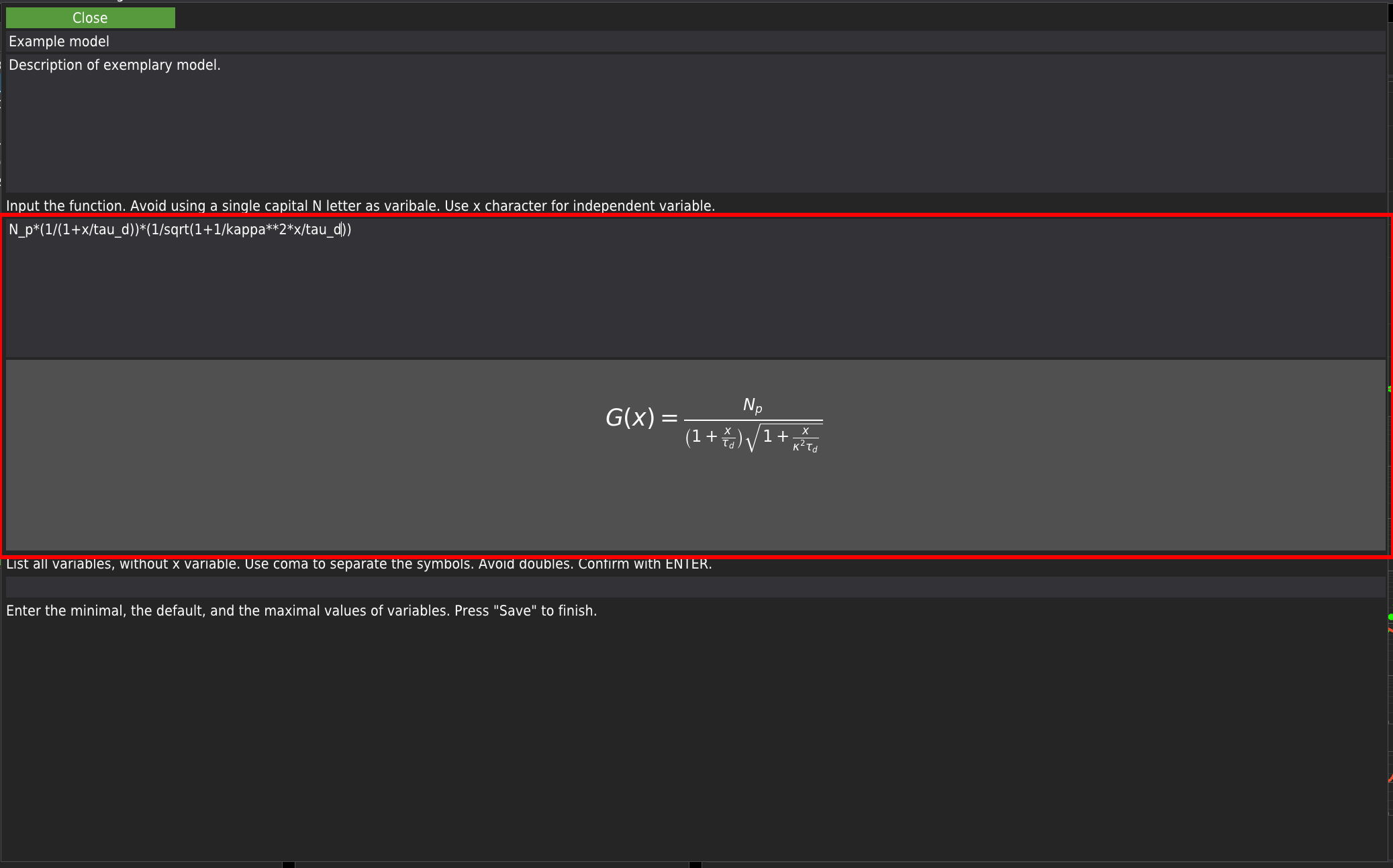
In the first two fields, at the top of the window, the user needs to provide the model’s name and a short description. Next, the equation describing the model should be provided. The edited equation is rendered on the flight in the field below. Due to technical reasons, avoid using capital N while editing the equation. The underscore mark can be used for indices. The power operation should be provided in a Python notation - a double asterisk character (**) instead of the caret (^) character. All operators should be provided, including the multiplication operator marked by the asterisk character. Use x as the independent variable. Note that the equation will not update if an error in the equation formula is detected. In the screenshot below, you can see an example input.
Before the provided model is added to the library, the software will double-check the variables used in the model’s equation. For this purpose, the user is asked to provide a list of variables (separated by commas and excluding the x variable). If the user-provided list of variables matches the list of variables extracted from the user-defined model’s equation, a set of editable fields labelled with the variable names will appear at the bottom of the window.
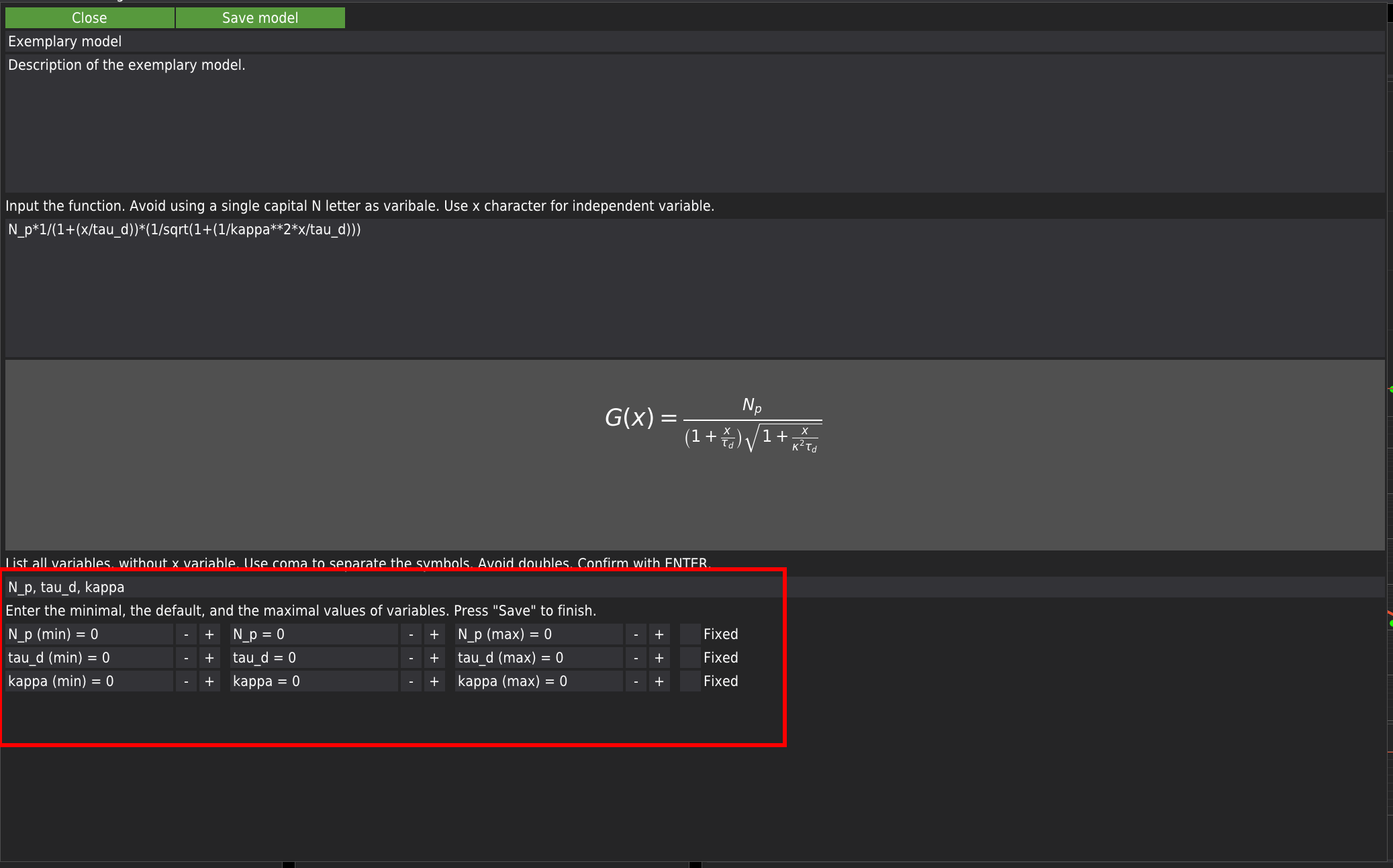
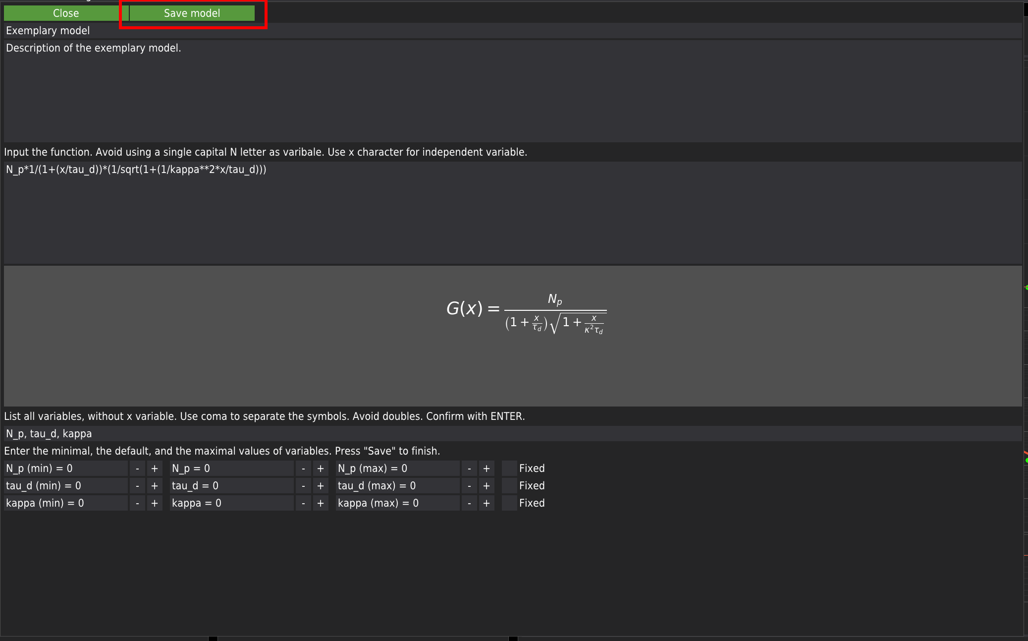
Here, the user is advised to provide the minimum expected value, the initial value, and the maximum expected value. All fields need to be filled. Keeping the default zero values can lead to fitting errors. Each variable has a checkbox marked as Fixed. By default, if the checkbox is checked, the variable will be kept constant during fitting. If the list of user-provided variables agrees with the list of variables extracted from the model’s equation, the Save model button will appear. Press it to add the model to the library. The user-defined model will appear in the list of models and will be labelled as User-defined -.
Controlling FCS data display
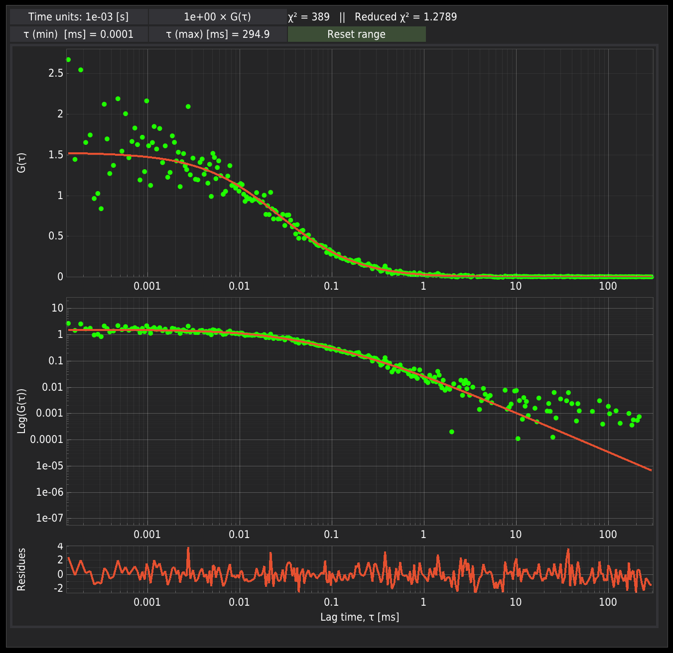
The FCS data and the corresponding function described by the model are depicted on the right panel. The data are displayed in two ways: the semi-log scale, which is the standard way the FCS data are displayed, and the log-log scale.
Above the plots, there are fields controlling the display of the FCS data:
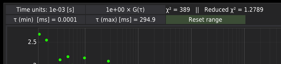
Time Units - this field defines the time scale at which the data are read from the files. This field should be used with great care. It is only useful when the data are imported from ASCII files generated by software that automatically scales the data. The user needs to be sure what time units are used in their data files. By default, the data are displayed in ms.
The multiplication factor. This field is only useful when the data are imported from the ASCII files generated by software that automatically scales the data. It may happen that the acquisition software (e.g., SymPhoTime64) exports the FCS data multiplied by 10-3. In those cases, this field is supposed to rescale the data to correct the value.
The text field displaying the and reduced values. The field appears after fitting.
(min) and (max) sliders. Those two fields allow the lag time range to change. Changes in the values affect the range of data used for fitting.
The reset range button sets the original range of the data. The button becomes active only after using the (min) or (max) sliders.
Fitting FCS data
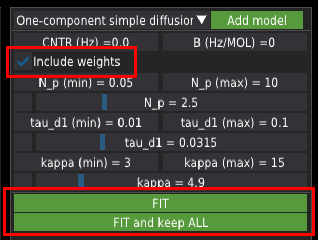
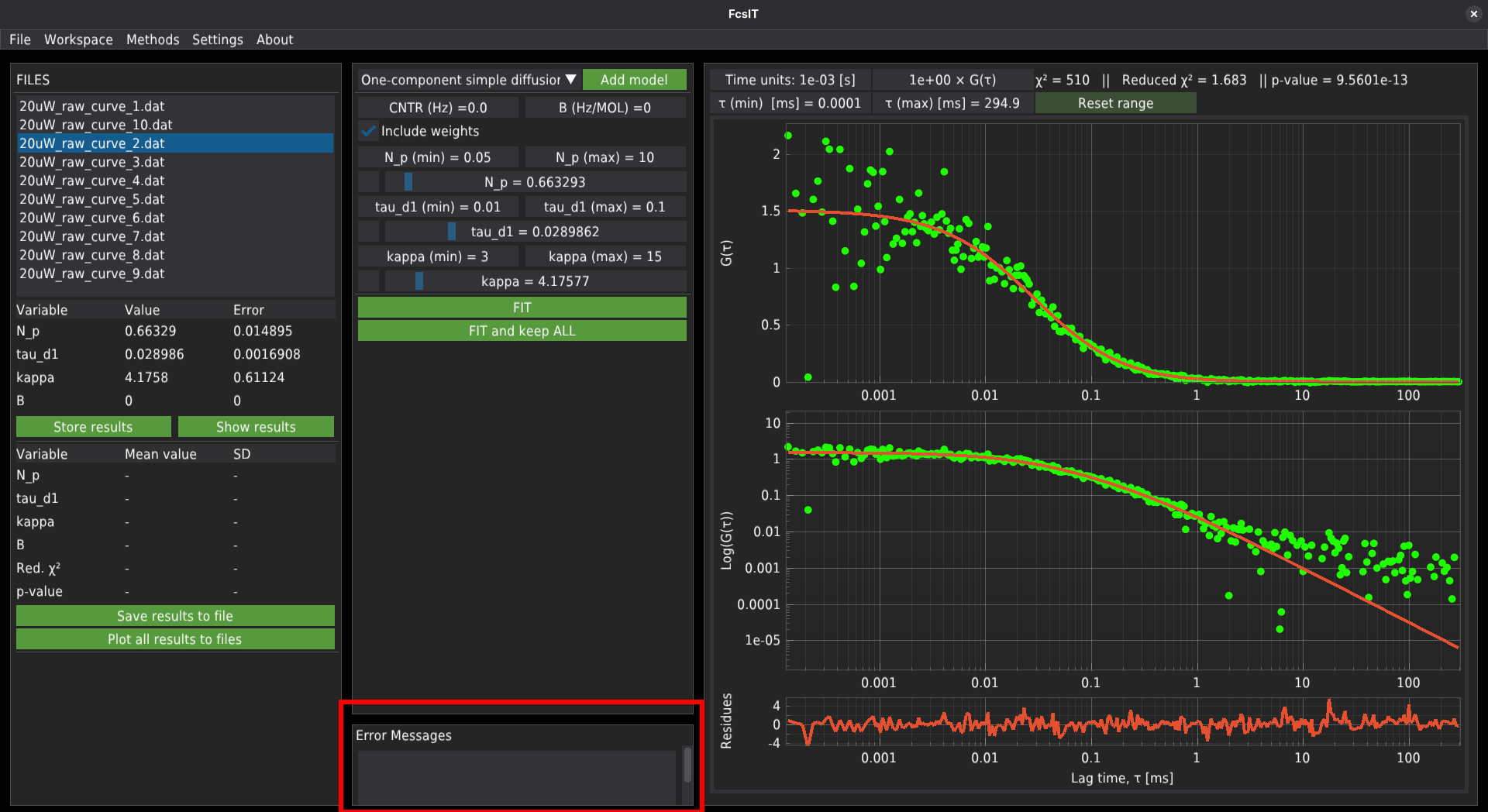
To fit the single file, press the FIT button. To fit all files from the list, press the FIT and keep ALL button. By default, the fitting algorithm will include weights (as the inverse of the error ) from the data file. The user can switch off this option by unchecking the Include weights checkbox.
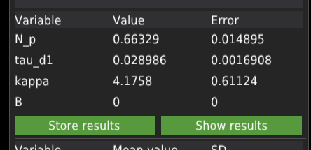
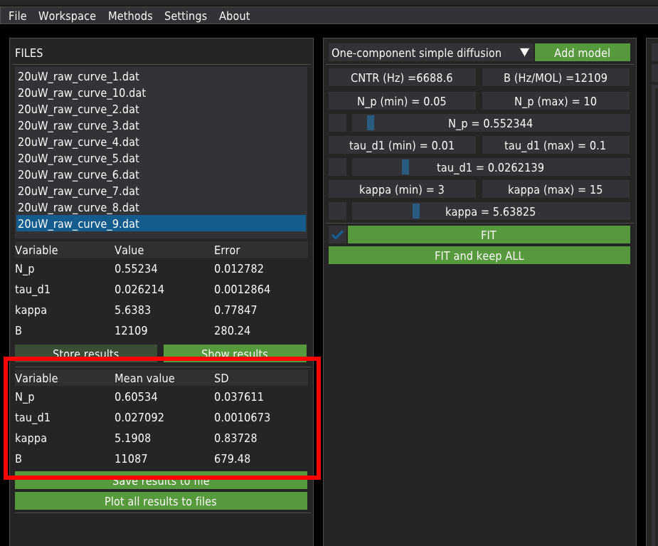
When a single file is fitted, the results are displayed in the table on the left panel.
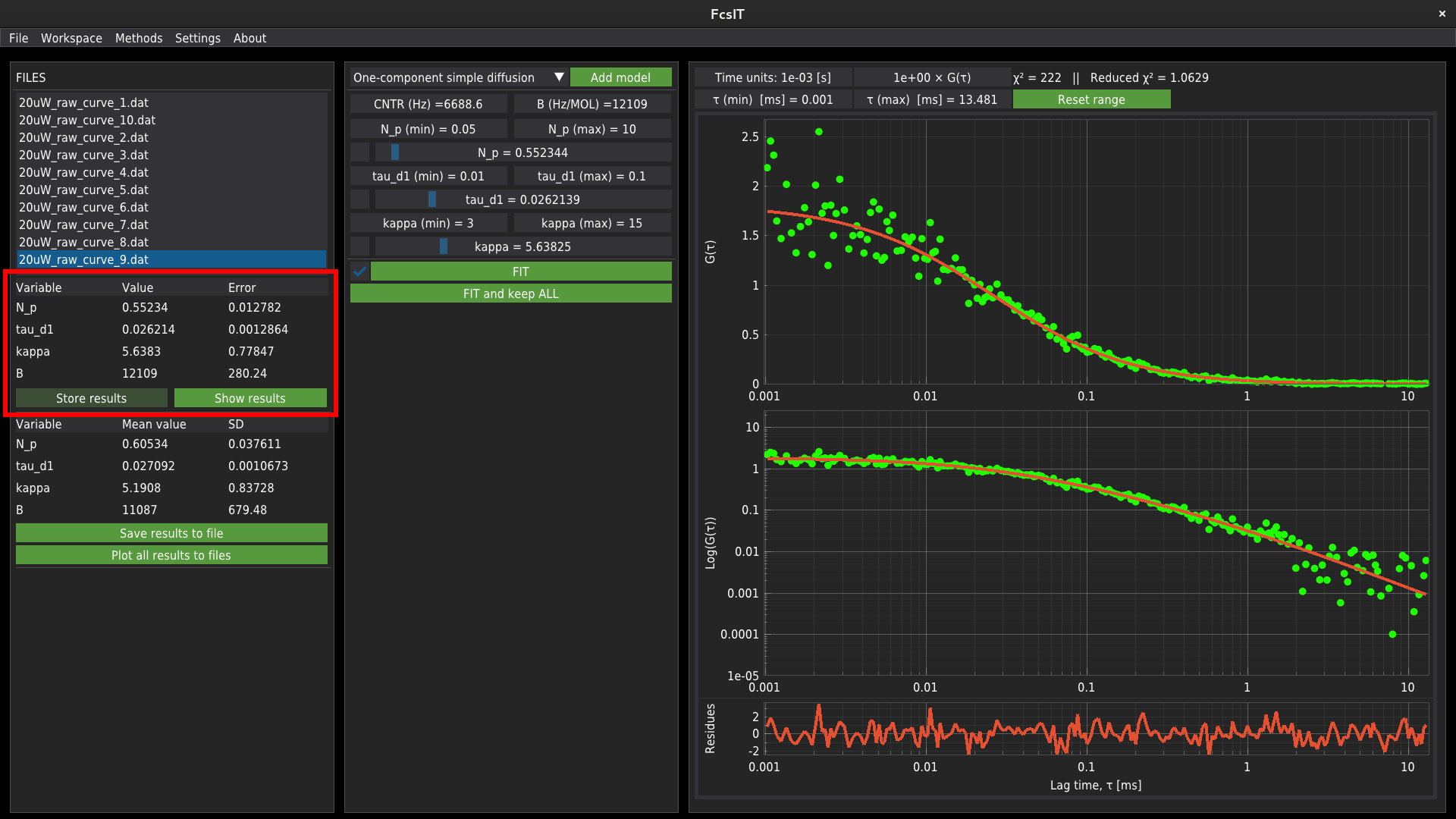
The user needs to manually add the results to the results database. Press Store results to add the results data.
When the FIT and keep ALL button was pressed to fit the data, the software would fit the curve and automatically add the results to the database. In some cases, the fitting algorithm may not find proper values. In such cases, the software will report an error in fitting a given file, which will appear in the Error Messages window at the bottom of the central panel. Clicking the record displayed in that window will automatically jump to the file. Then the user can adjust the initial parameters and fit the single file. If the fit succeeds, the error message will disappear. In that case, the data needs to be stored manually which may lead to double te reusults records in the database.
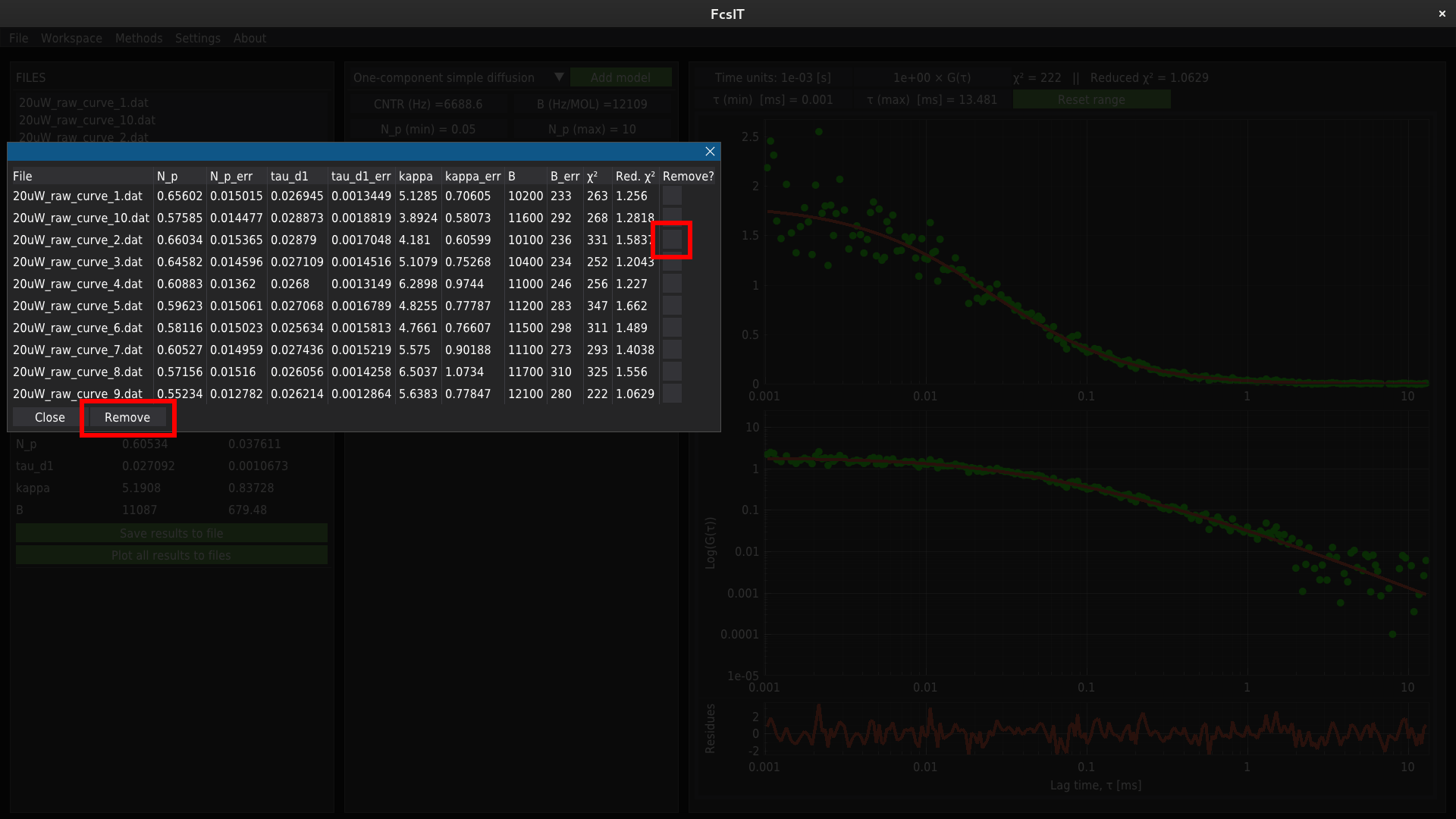
The database of all fitted files can be viewed (and, if necessary, removed from the database) by pressing the Show results button.
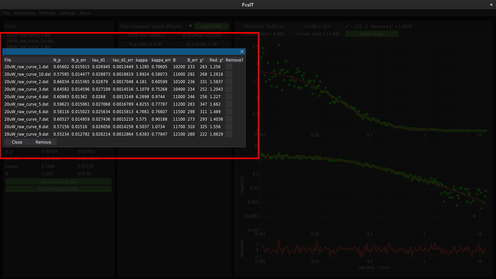
To remove the record from the results database, selct required row by using the checkboxes on the right side of the table. and click Remove button.
The mean values of fitting parameters for all fitted files are displayed in the lower table on the left panel.
Export results
To export the results, press the Save results to file button; this opens a dialogue to choose the output file path and filename. By default, the file name is results. The data can be stored in one of two formats:
.csv - a text format,
.pickle - a binary format in the form of the pandas DataFrame.
Additionally, clicking the Plot all results to files button opens a dialogue to select a folder to store the plotted data. The plots of all fitted files will be stored as .png files. The other formats, including the text data and binary pandas DataFrame, are available to set in the Settings menu.