Extract from PTU and filter
Import PTU files
First, click “File” and “Open PTU directory” to select the folder storing your .ptu files.
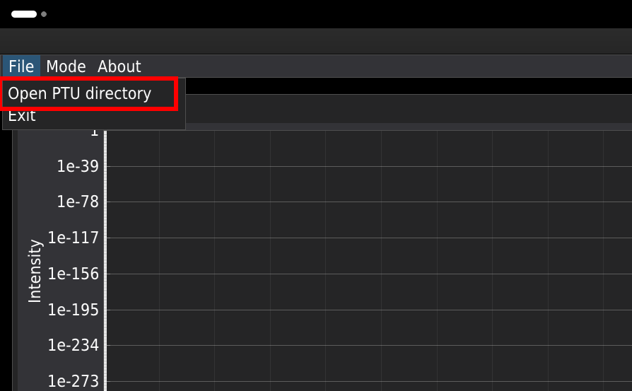
We suggest keeping the .ptu files for a single experiment in a dedicated folder, one folder per experiment. The lifetime analysis can be performed for each channel separately.
The main window
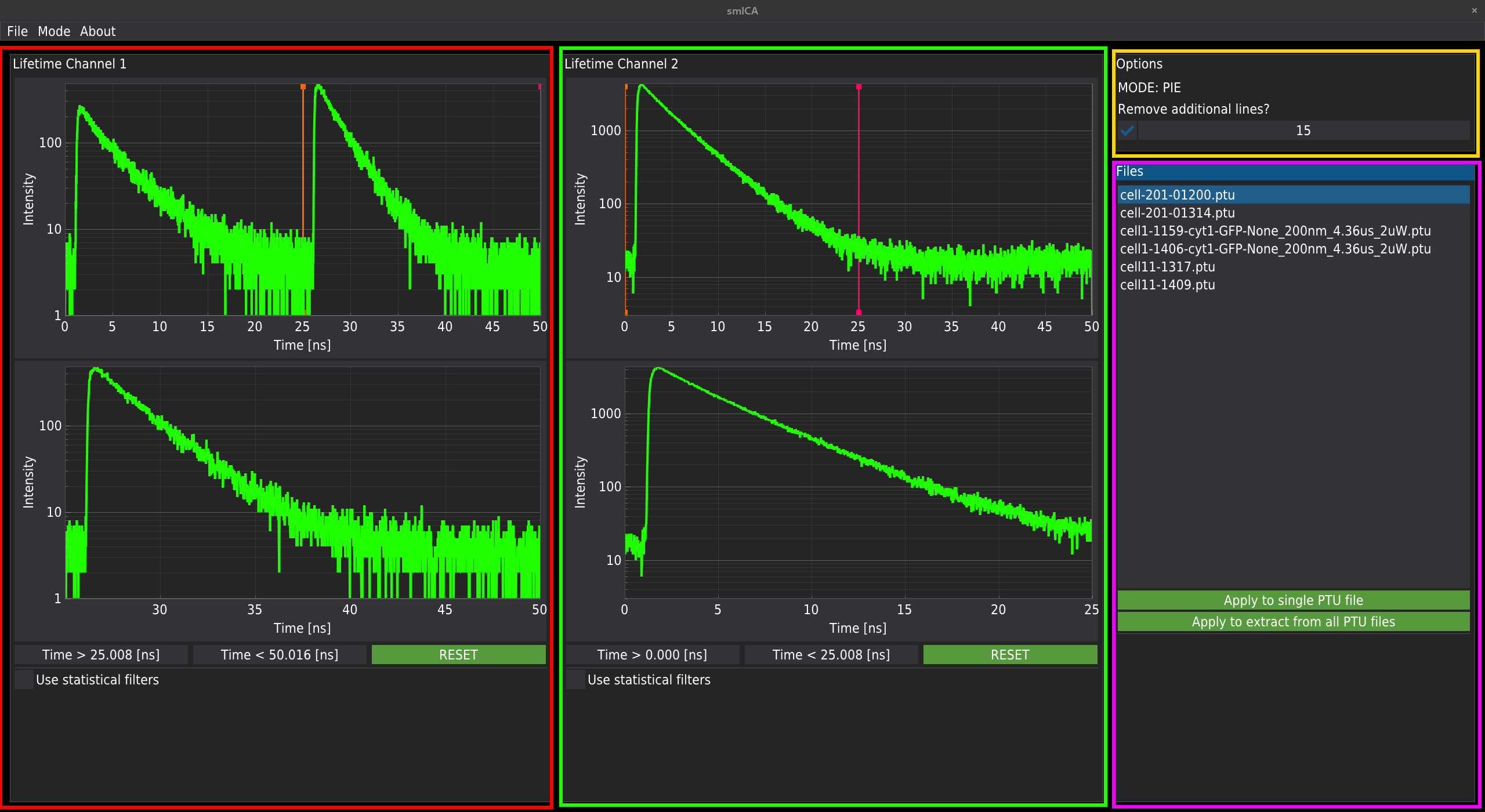
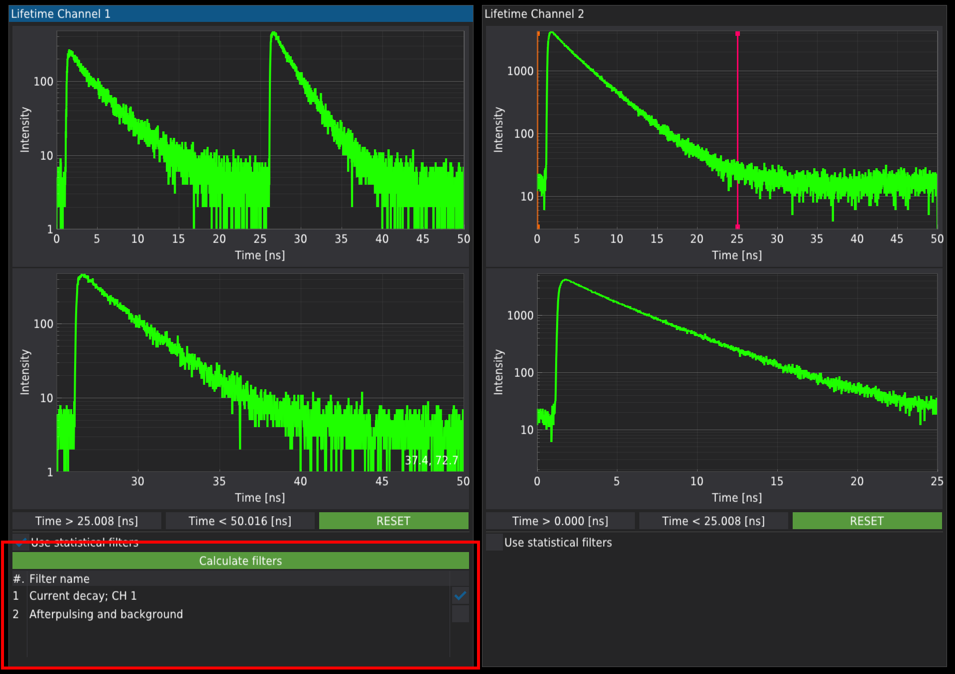
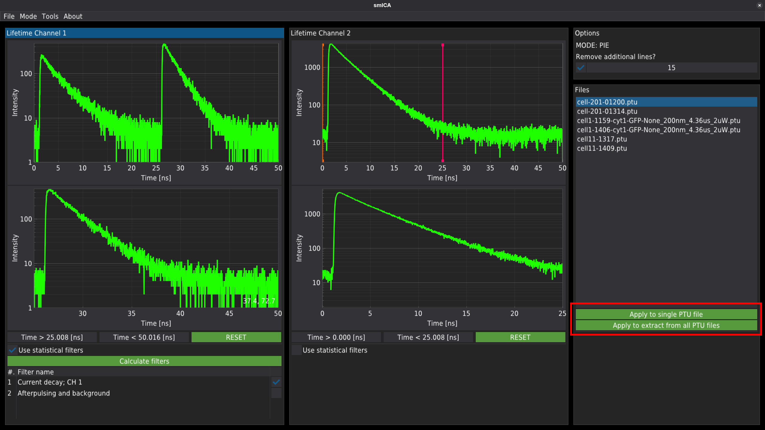
The main window of the method is composed of four sub-windows. If two detectors are used in the measurement, the signal will be automatically split and displayed as Channel 1 (red) and Channel 2 (green). The upper plots represent the whole signal acquired by a given detector. The lower plot displays only the parts of the signal selected by the draglines in the upper plots. The script recognises the measurement mode (standard or PIE). If the PIE mode is enabled, the draglines will automatically split the entire time range in half. Only the signal from the lower plots will be used for analysis.
Important! Some older hardware based on NIKON A1 and LSM upgrade kits from PicoQuant may experience a hardware communication bug between the A1 controller and the SymPhoTime software during .ptu file acquisition. Due to a bug, additional lines are added to the figure generated by SymPhoTime, resulting in a smeared appearance at the top of the figure. The panel marked with a yellow rectangle in the top-right corner of the main window lets you enable correction for additional lines.
The magenta rectangle marks the window containing all files from the selected folder, along with buttons to run the analysis for a single file or all files.
Filtering the data
The software allows for two types of photon filtering. Each channel can be filtered independently.
Time gating
The first filtering method uses simple time gating. It can be realised by selecting the region of interest in the fluorescence decay pattern by moving the orange and red drag lines displayed in the upper plots.
TCSPC filtering
The second method is based on statistical TCSPC filtering, in which proper weights are assigned according to the procedure described in the literature (see Enderlein & Gregor (2005) and Kapusta et al. (2007)). Below is the step-by-step filtering procedure.
Checking the “Use statistical filters” checkbox under each channel deactivates draglines and activates
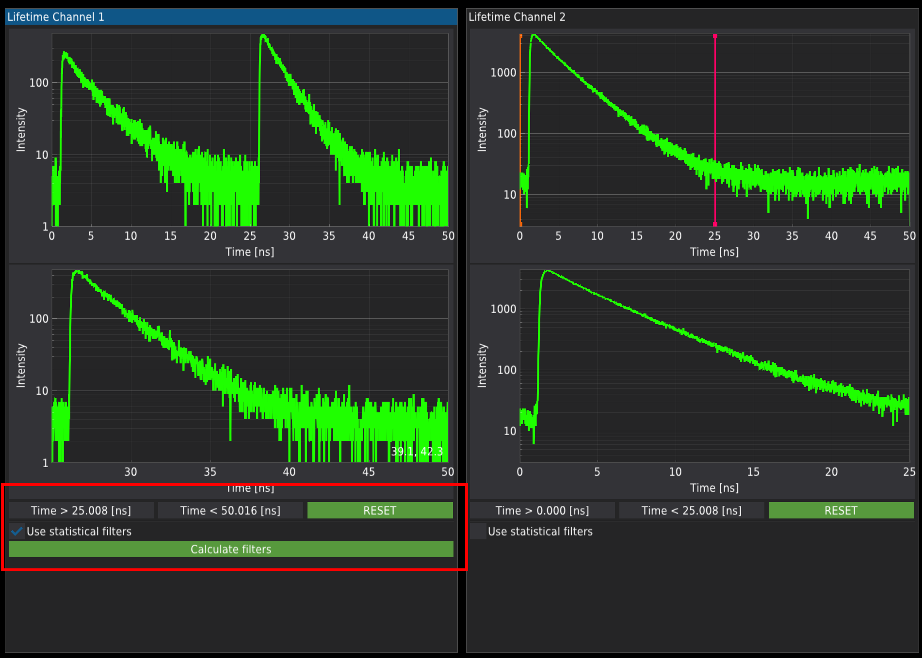
Define pattern
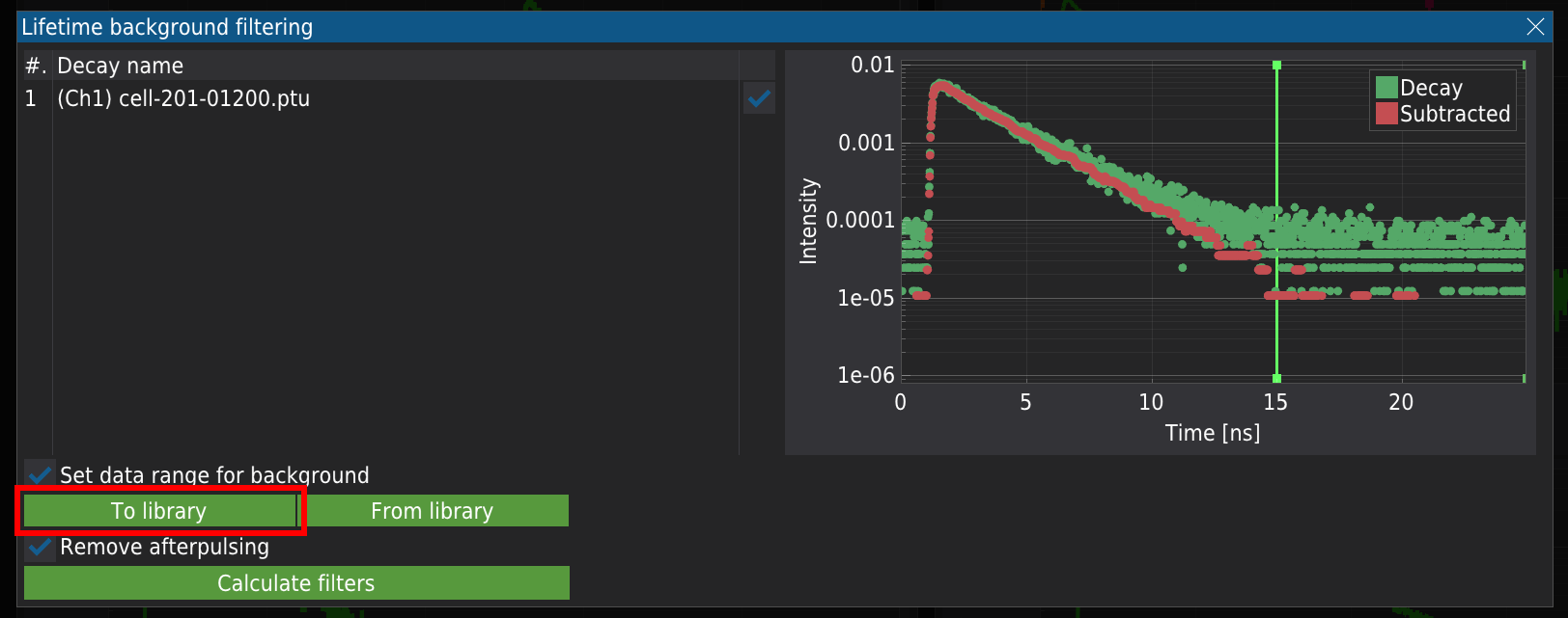
The “Calculate filters” opens a window (see below) where the user can calculate statistical filters for background or fluorescence decay patterns imported from the library.
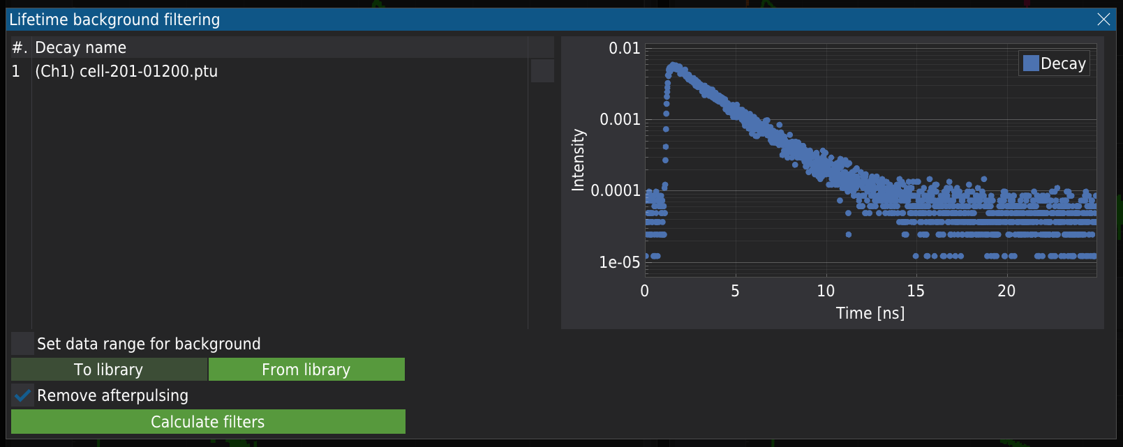
On the left of the above window is a list of decay patterns. Initially, only one pattern appears, corresponding to the pattern extracted from the image at a given channel, the one from the plot.
Selecting the “Set data range for background” checkbox activates draglines, allowing one to select the background region of the pattern, usually the plateau at the highest times of the decay pattern. Based on the selected region, the mean background signal is calculated and subtracted from the original decay data. The subtracted data is then used to calculate the statistical filter. altervnatively the filtering pattern can be stored in the library by pressing “To library”.
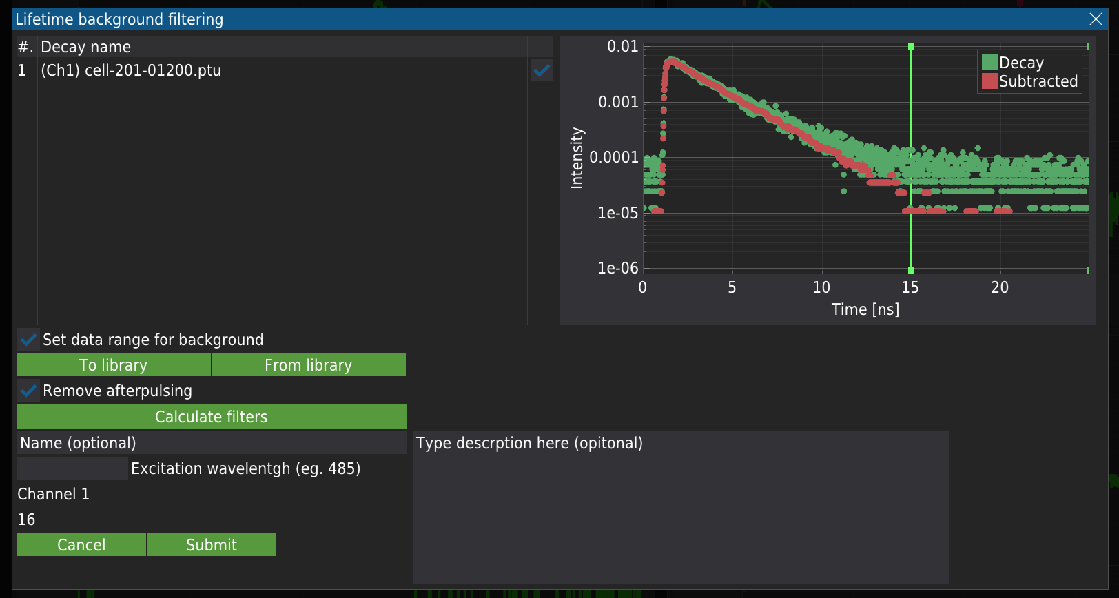
Adding pattern to library
The background-free decay pattern can be stored in the library for later use. Press “To library”. To add the the pattern to the library.
The new fields will appear, which are required to store the data. Although some fields are optional, the more details you provide, the easier you will find the proper decay. To store the data, press “Submit”.
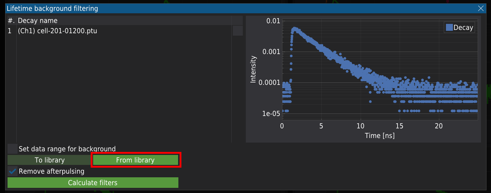
Import the decay pattern from the library
The previously stored decay data can also be imported by pressing the “Form library” button.
The new table will appear, containing all the stored decay patterns. Marking the decay and pressing “Import” will load the decay pattern.
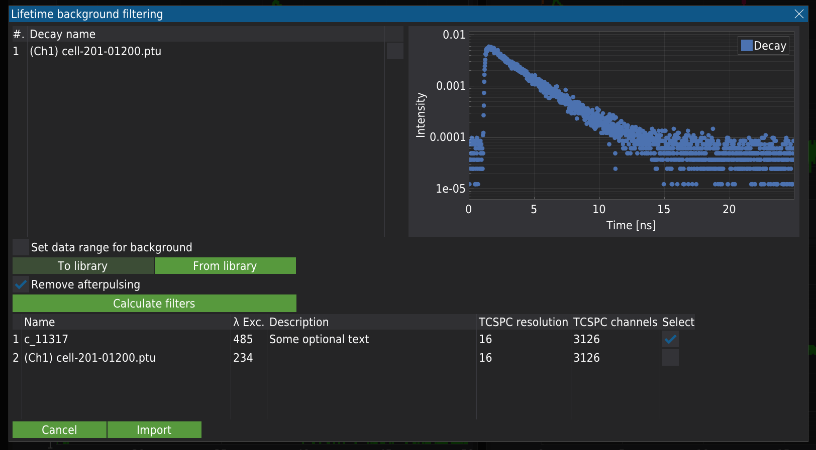
Calculate filters
For data imported from the library, the user needs to select the appropriate pattern required for the analysis. When only background removal is performed, it is recommended to select the “Remove afterpulsing” checkbox.
Pressing the “Calculate filters” button calculates weights, which are displayed in a new plot. Note that the calculations can take some time. The plot displays all the weights calculated for the curves in the left table, together with the background and afterpulsing signal. To accept the current set of weights, press “Accept”; to reject and recalculate, press “Decline”.
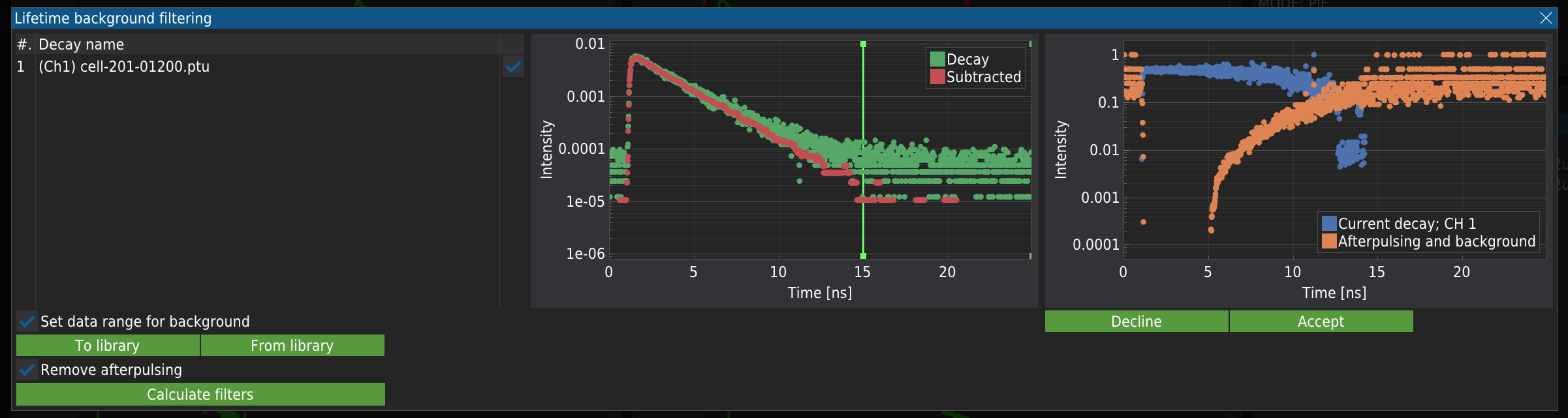
The “Accept” button will close the window, and you can select the weights for analysis. Make sure you select the proper weights. For example, selecting the Afterpulsing and background weights will remove your fluorophore’s signal, and for the analysis, only the background signal will be used.
The same procedure can be repeated for Channel 2.
Apply the filtering routine
Finally, pressing one of the buttons labelled Apply to single PTU file or Apply to extract from all PTU files will run a filtering routine on a single selected file or on all files in the directory.
Output
Every time the filtering routine is applied, the script generates several files for further analysis. The files will be named after the used _ .ptu _ file.
The script will generate:
some-file.pkl - The binary file containing experimental data. The file is necessary to generate the concentration map.
Two .png files per channel. One in the normalised grey scale and one in the false colours mode, where the intensity of fluorescence is mapped with different colours.
The .pkl file is a pickle file containing the Python dictionary. The file structure is described in the table below.
| Keys | Value description |
|---|---|
| File info | The Python dictionary containing: |
| ‘L_file’ : name of the .ptu_file | |
| ‘Pixels per line’: number of pixels in a line in the image | |
| ‘Number of lines’: number of lines in the image | |
| ‘Pixels size’: size of the single pixel (nm) | |
| ‘Number of frames’: number of frames acquired during the single measurement | |
| ‘Pixel dwell’ : The time in s that is spend to illuminate a single pixel | |
| ‘Lifetime resolution’: The temporal resolution of the fluorescence decay (ns) | |
| export_df_1 | The pandas DataFrame containing the number of photons registered in channel 1 for each pixel |
| export_df_2 | The pandas DataFrame containing the number of photons registered in channel 1 for each pixel |
| taus_1 | The pandas DataFrame containing the TCSPC histogram registered in channel 1. The time-gated signal |
| taus_2 | The pandas DataFrame containing the TCSPC histogram registered in channel 2. The time-gated signal |
| fulltaus_1 | The pandas DataFrame containing the full TCSPC histogram registered in channel 1. |
| fulltaus_2 | The pandas DataFrame containing the full TCSPC histogram registered in channel 2. |
| lifetimes_1 | Numpy array containing the fluorescence lifetime for each pixel registered in channel 1. Signal after time-gating/filtration. |
| lifetimes_2 | Numpy array containing the fluorescence lifetime for each pixel registered in channel 2. Signal after time-gating/filtration. |
| intensity_1 | Numpy array containing the number of photons for each pixel registered in channel 1. Signal after time-gating/filtration. |
| intensity_2 | Numpy array containing the number of photons for each pixel registered in channel 2. Signal after time-gating/filtration. |
| bgrnd_1 | Numpy array containing the filtered background registered for channel 1. |
| bgrnd_2 | Numpy array containing the filtered background registered for channel 2. |
| filter_weight_1 | Numpy array containing the weights for each TCSPC channel calculated for channel 1. |
| filter_weight_2 | Numpy array containing the weights for each TCSPC channel calculated for channel 2. |
| filter_afterpulsing_weight_1 | Numpy array containing the weights for each TCSPC channel calculated for the background for channel 1. |
| filter_afterpulsing_weight_2 | Numpy array containing the weights for each TCSPC channel calculated for the background for channel 2. |
| special_markers_1 | Pandas dataframe containing full TCSPC information for both channels. |
| special_markers_2 | Duplicated from special_markers_1 |
| filtered_taus_1 | Pandas dataframe containing the TVSPC histogram after the TCSPC filtration procedure for channel 2. |
| filtered_taus_1 | Pandas dataframe containing the TVSPC histogram after the TCSPC filtration procedure for channel 2. |
| The minimal Python script to get the pickled data is below. |
    import os
    import pickle
    import pandas as pd
    import numpy as np
    path = '<path-to-file>/<file-name>.pkl'

    with open(path, 'rb') as file:
        pkl = pickle.load(file)

    file_info = pkl['File info']
    print(file_info)

    DF_1 = pkl['export_df_1']
    DF_2 = pkl['export_df_2']
    print(DF_1)
    print(DF_2)

    DF_taus_1 = pkl['taus_1']
    DF_taus_2 = pkl['taus_2']

    print(DF_taus_1)
    print(DF_taus_2)

    DF_ftaus_1 = pkl['fulltaus_1']
    DF_ftaus_2 = pkl['fulltaus_2']

    print(DF_ftaus_1)
    print(DF_ftaus_2)

    lifetimes_1 = pkl['lifetimes_1']
    lifetimes_2 = pkl['lifetimes_2']

    print(lifetimes_1)
    print(lifetimes_2)

    intensity_1 = pkl['intensity_1']
    intensity_2 = pkl['intensity_2']

    print(intensity_1)
    print(intensity_2)

    bgrnd_1 = pkl['bgrnd_1']
    bgrnd_2 = pkl['bgrnd_2']

    print(bgrnd_1)
    print(bgrnd_2)

    filter_weight_1 = pkl['filter_weight_1']
    filter_weight_2 = pkl['filter_weight_2']

    print(filter_weight_1)
    print(filter_weight_2)

    filter_afterpulsing_weight_1 = pkl['filter_afterpulsing_weight_1']
    filter_afterpulsing_weight_2 = pkl['filter_afterpulsing_weight_2']

    print(filter_afterpulsing_weight_1)
    print(filter_afterpulsing_weight_2)

    special_markers_1 = pkl['special_markers_1']
    special_markers_2 = pkl['special_markers_2']

    print(special_markers_1)
    print(special_markers_2)

    filtered_taus_1 = pkl['filtered_taus_1']
    filtered_taus_2 = pkl['filtered_taus_2']

    print(filtered_taus_1)
print(filtered_taus_2)- Enderlein, J., & Gregor, I. (2005). Using fluorescence lifetime for discriminating detector afterpulsing in fluorescence-correlation spectroscopy. Review of Scientific Instruments, 76. 10.1063/1.1863399
- Kapusta, P., Wahl, M., Benda, A., & Hof, M. (2007). Fluorescence lifetime correlation spectroscopy. Journal of Fluorescence, 17, 43–48. 10.1007/s10895-006-0145-1